
other Handouts



|
|
|
other Handouts
|
|
|
|
Textbook
|
Title
|
Duration
|
Link
|
Description |
|
-
|
17:41 | General advice for students starting a college level mathematics course. Appropriate for students starting calculus. | ||
|
-
|
17:03 | A brief overview of the main themes of calculus. What to expect from a typical three-course calculus sequence. | ||
|
-
|
13:43 | This is how I try to explain limits to someone who hasn't taken calculus before. | ||
|
§ 3.11
|
6:39 | Introduction to calculus problems regarding related rates (word problems using the chain rule). We discuss the setup; subsequent videos give examples. | ||
|
§ 3.11
|
11:50 | A first example of related rates: Air is pumped into an inflatable balloon at a rate of 10 in^3/sec. How fast is the diameter increasing at the moment when the diameter is (a) 5 in; (b) 10 in? | ||
|
§ 3.11
|
8:24 | Continuing our example of a first related rates problem in calculus | ||
|
§ 3.11
|
15:03 | We discuss three slightly different solutions to the following related rates problem: An airplane flies due west at an altitude of 1mi. Shortly after passing directly over our heads, it passes over the nearest town 1.4 miles to our west. Assuming the plane has groundspeed 540mph at that instant, how fast is the plane receding from us? | ||
|
§ 3.11
|
10:33 | Sequel to our previous video, Airplane I. Here we solve another related rates problem in calculus: An airplane is 1.4mi due west of us, flying due west at an altitude of 1mi. We observe its angle of inclination above the horizon. Assuming its groundspeed at that instant is 540mph, what is the rate of change of the angle of inclination? | ||
|
§ 3.11
|
||||
|
§ 4.1
|
Maxima and Minima | 23:08 | 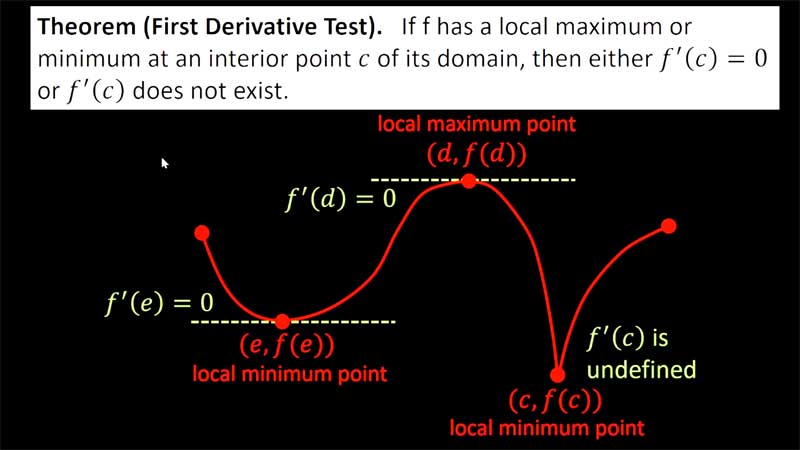 |
We introduce the notion of extrema (maxima and minima) for functions in single-variable calculus. |
| § 4.2 | Mean Value Theorem I | 8:30 | 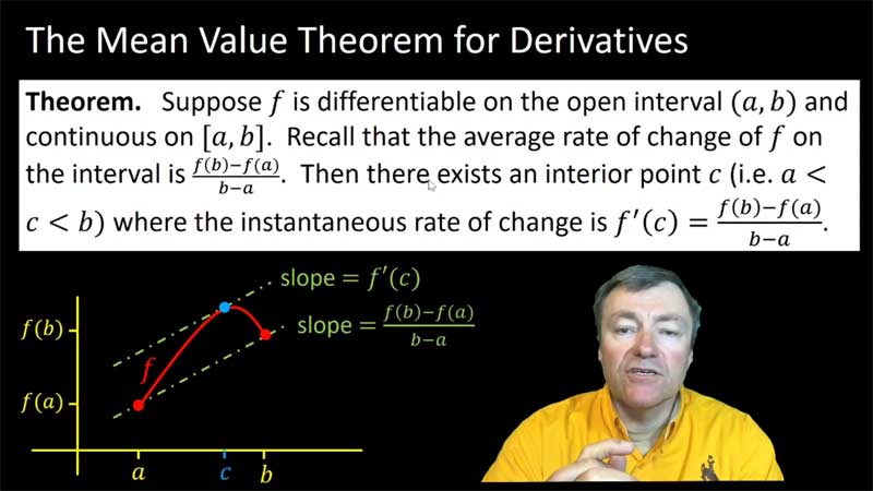 |
The Mean Value Theorem for Derivatives (together with Rolle's Theorem) are introduced. |
| § 4.2-4.3 | Mean Value Theorem II | 13:34 | 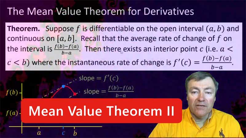 |
The Mean Value Theorem is used to test when a function is constant (or increasing or decreasing). We also discuss when two functions can have the same derivative. |
| § 4.3 | The Derivative Tests | 27:44 | 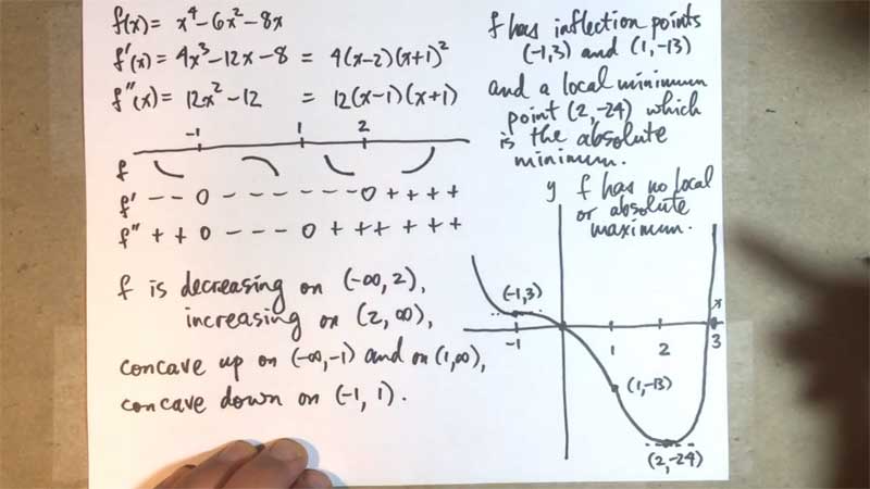 |
The First and Second Derivative Tests are introduced, whereby we determine intervals where a graph is increasing or decreasing, concave up or concave down. Example 1 (at 8:11) considers |
| § 4.3 | Some Fabulous Polynomials | 12:48 |  |
A remarkable sequence of polynomials is exhibited. Using the First Derivative Test, it is easily shown that these polynomials give lower bounds for ex (for x > 0). An application is given to evaluating certain limits. |
| § 4.4 | Sketching Graphs I | 13:10 |  |
We apply tools from calculus together with tools from pre-calculus in the art of sketching graphs of functions. At 6:27 we demonstrate using f(x)=(x2+36)/2x. |
| § 4.4 | Sketching Graphs II | 7:17 | 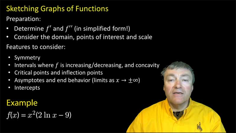 |
As a second example, we sketch the graph of f(x)=x2(2ln(x)-9). |
| § 4.5 | The Largest Box | 5:11 | 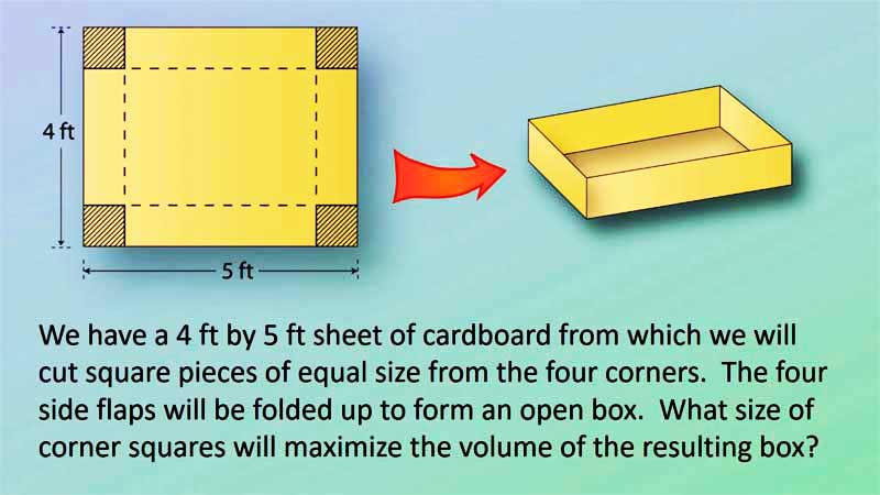 |
From a 4ft by 5ft sheet of cardboard, we cut squares of equal size from the four corners. This leaves four flaps on the sides which fold up to yield a box with an open top. What size of square cutouts from the corners will maximize the volume of the resulting box? |
| § 4.5 | The Shortest Ladder | 7:11 | 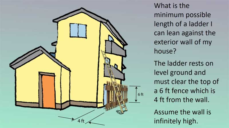 |
We want to lean a ladder against the outside wall of our house. What is the shortest possible ladder we can use if the ladder must reach over the top of a 6 ft tall fence which is 4 ft from the wall? |
| § 4.6 | Linearization and Differentials | 22:05 | 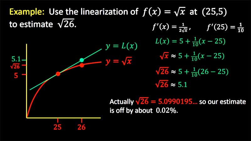 |
We discuss the linear approximation to a function at a point of its graph. At 12:05 we introduce differentials and discuss several ways they are used. |
| § 4.7 | l'Hôpital's Rule | 25.59 |  |
We explain how l'Hôpital's Rule is used to evaluate limits of indeterminate forms. Many examples (having different indeterminate forms) are included. |
| § 4.7 | Why the interest in e? | 12:31 |  |
The exponential function ex and the natural base e are shown to arise naturally in the context of continuously compounded interest. This uses l'Hôpital's Rule to resolve yet another indeterminate form. |
| § 4.9 | Antiderivatives I | 23:27 |  |
Antiderivatives are introduced. If f is the derivative of F (i.e. F′ = f ) then F is an antiderivative of f. |
| § 4.9 | Antiderivatives II | 15:02 | 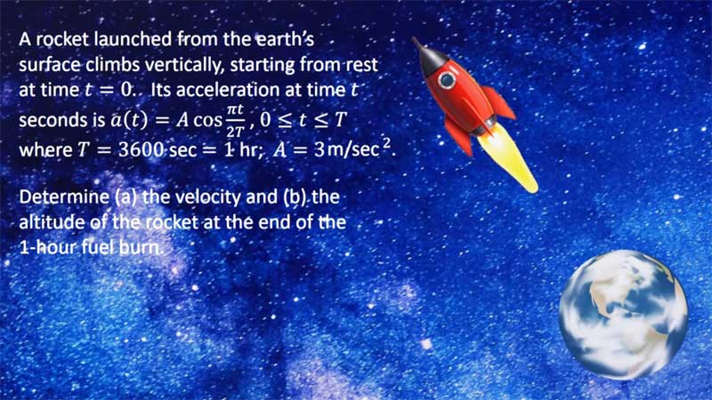 |
We continue discussing antiderivatives. At 5:25 we solve a problem: A rocket launched from the Earth's surface climbs vertically, starting from rest at time t=0. Its acceleration at time t seconds is a(t)=A cos(πt/2T) where T=1 hr and A=3m/sec2. Determine (a) the velocity and (b) the altitude of the rocket at the end of the 1-hour fuel burn. |
| § 5.1 | Riemann Sums I | 26:34 | 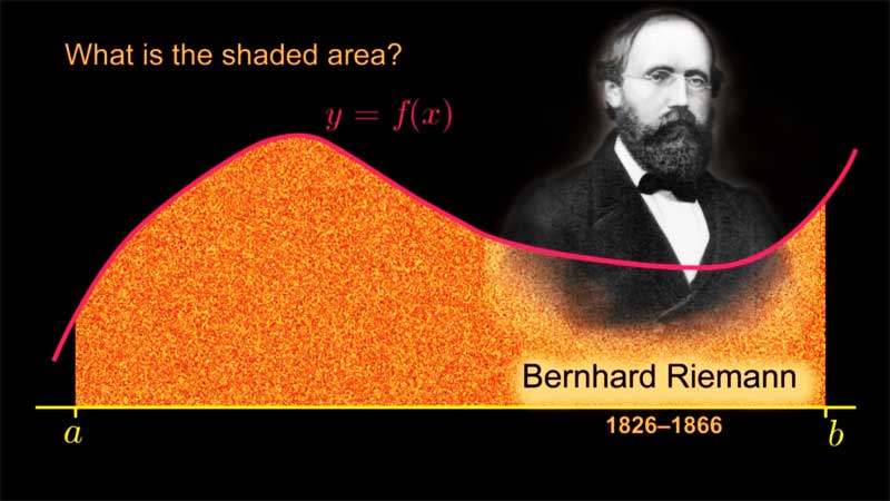 |
We introduce Riemann sums as approximations to areas under curves; and by taking the appropriate limit, we arrive at the definition of a Riemann integral. |
| § 5.1 | Riemann Sums II | 6:23 | 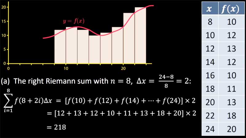 |
Using a table of values for a function, we compute left, right and midpoint Riemann sums using n=8,8,4 subintervals respectively. |
| § 5.1 | Riemann Sums III | 8:52 | 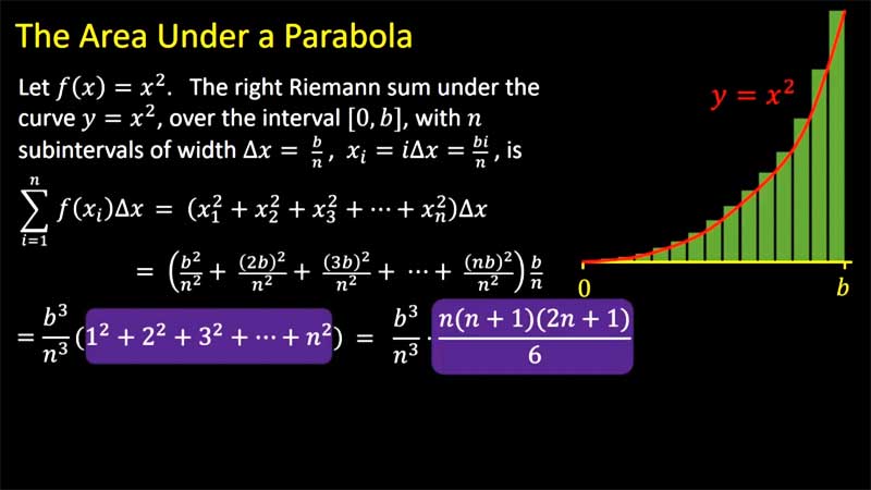 |
We evaluate two integrals using the definition (as the limit of Riemann sums) just for the functions f(x)=x and x2. |
| § 5.2 | Integrals | 13:52 | 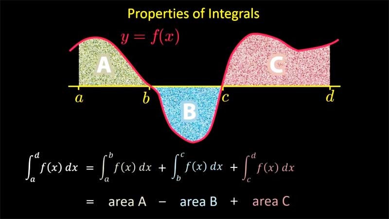 |
We cover the most basic properties of integrals, and their relationship with area. |
| § 5.3 | Fundamental Theorem I | 13:28 | 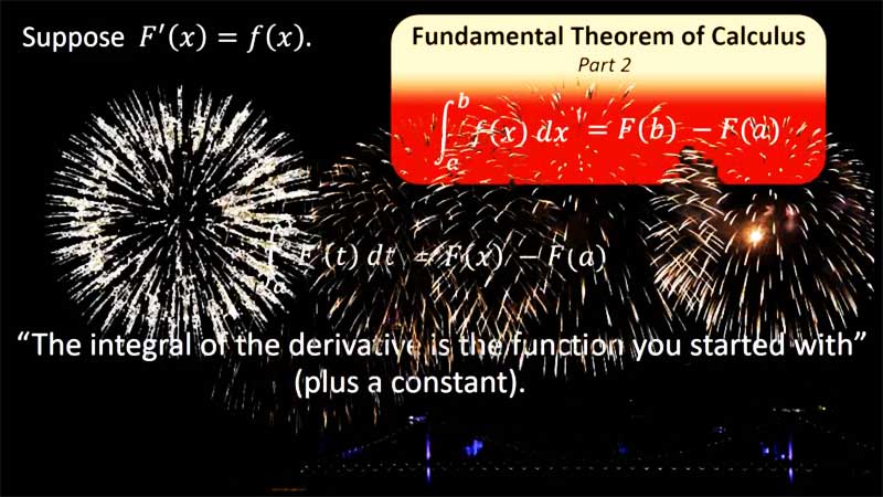 |
The Fundamental Theorem of Calculus is introduced in both its forms. |
| § 5.3 | Fundamental Theorem II | 11:36 | 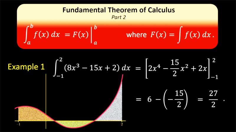 |
Examples using Part 2 of the Fundamental Theorem of Calculus. |
| § 5.3 | Fundamental Theorem III | 13:01 | 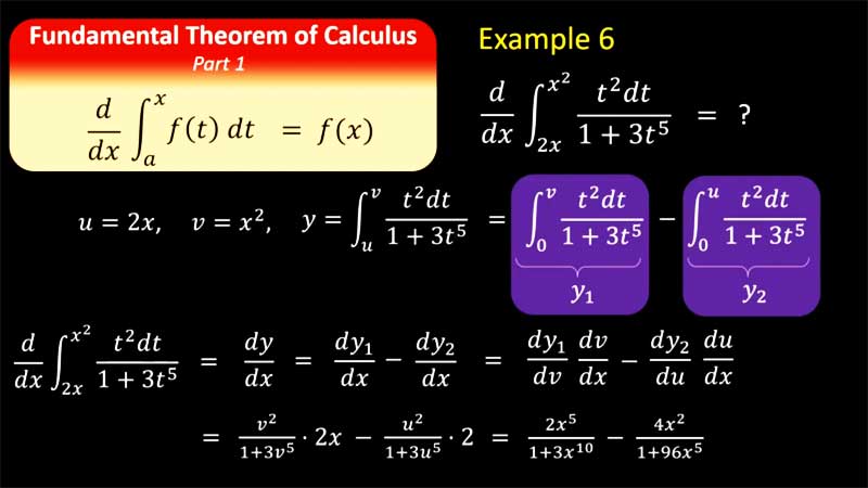 |
Examples using Part 1 of the Fundamental Theorem of Calculus. |
| § 5.4 | Average Value of a Function | 18:51 |  |
We define the average value of a function on an interval. We also discuss the use of symmetry in computing integrals. |
| § | ||||
| § |
| Yellow rows feature content from the textbook. I may ask you questions directly about this material. | Green rows feature content not taken directly from the textbook. I won't expect you to answer questions directly on this material. But I expect you to learn this because it provides background and context which is helpful for the core material. |
|
Textbook
|
Title
|
Duration
|
Link
|
Description |
|
-
|
17:41 | General advice for students starting a college level mathematics course. | ||
|
pp.1–4, 299–300
|
32:55 | We place the real numbers in the context of the zoo of important number systems. | ||
|
pp.32, 303
|
24:09 | Decimals are such a handy way to express real numbers... it's tempting to forget that the real number system is not defined using decimals. | ||
| pp.30, 36 | Equivalence Relations | 30:52 | 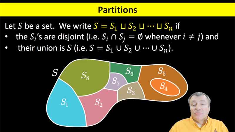 |
Equivalence relations serve as an extremely prolific tool for constructing new mathematical structures from old. |
| § | Complex Numbers | 15:27 | 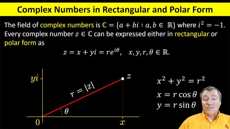 |
Much can be said about properties and applications of the complex numbers. Here we highlight some ways that the complex numbers shed light on the real numbers. |
| pp.145–148 | The Hierarchy of Smoothness | 20:01 | 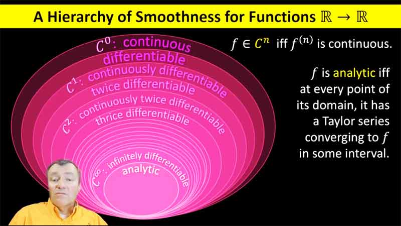 |
Functions from the reals to the reals are classified by their degree of smoothness, which is to say, how many times they can be differentiated. |
| § | Fabulous Polynomials | 12:48 |  |
This video features graphs of the first few Taylor polynomials for ex. Although the video was prepared for Calculus I students (who have not seen Taylor polynomials), the polynomials were introduced in a different way. |
| § | Polynomials and Series | 28:35 | 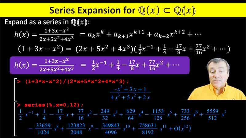 |
We introduce polynomials, rational functions, power series and Laurent series from a formal (i.e. symbolic) perspective. |
| pp.5–7 | Sets | 22:51 | 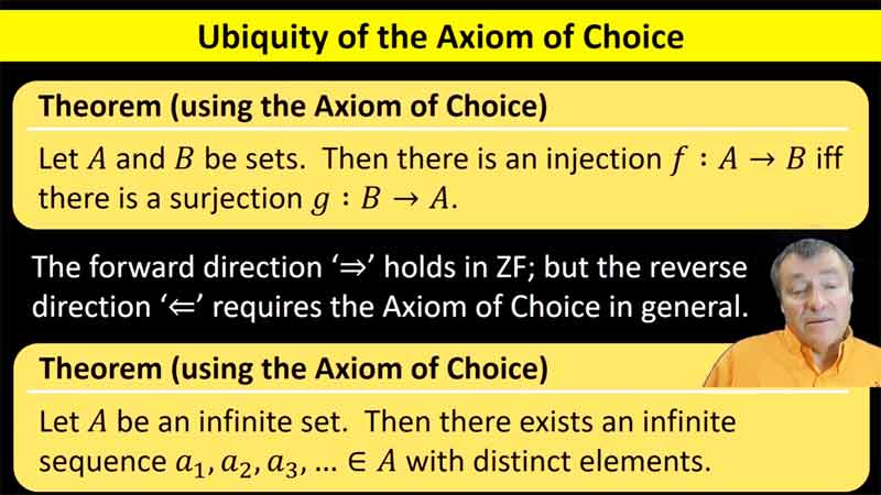 |
Russell's Paradox showed the need for axioms for set theory. Our standard axioms for modern set theory are ZF and ZFC. We don't list the axioms of ZF, but we do introduce the Axiom of Choice. |
| pp.25–32, 36–37 | Cardinality | 25:05 | 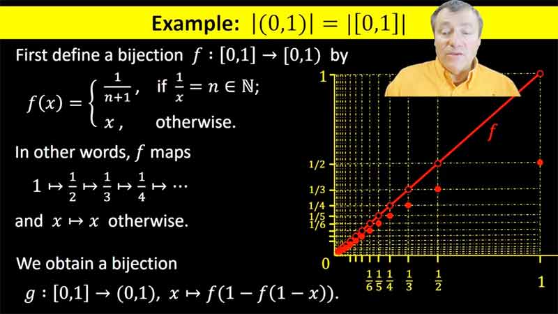 |
We discuss how an arbitrary pair of sets may be compared in size (as having the same size, or one has size greater than that of the other). In particular we discuss countability. |
| pp.32–35 | Uncountability | 38:30 | 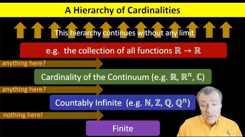 |
We present Cantor's theorems: The power set of any set is larger than the original set. In particular, the set of real numbers is uncountable. |
| pp.15–20 | Bounds | 21:47 | 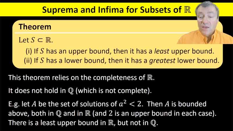 |
We talk about bounds for sets, including upper and lower bounds; also least upper bounds (suprema) and greatest lower bounds (infima). |
| Logic | 28:56 | 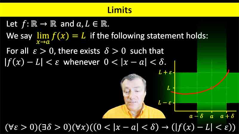 |
We discuss some of the logical language used in mathematical proofs, particularly in analysis. This includes a review of the definition of limits for univariate functions in calculus. | |
| Banach-Tarski | 12:19 |  |
We describe the Banach-Tarski Theorem as a way of providing our first hint of non-measurable sets; and a further reminder of the distinction between real numbers and physical reality. | |
| pp.20–21 | Nested Intervals | 12:02 | 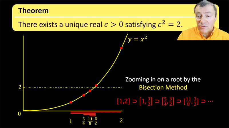 |
We prove the Nested Interval Theorem and use it to prove at 2 has a real square root. This example serves as a precursor to our later proof of the Intermediate Value Theorem. |
| pp.10–11 | Mathematical Induction | 24:08 | 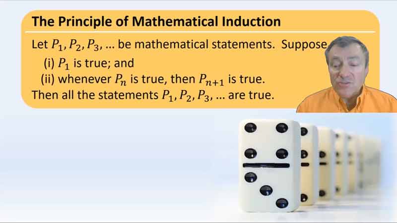 |
We introduce the Principle of Mathematical Induction, along with several examples. The Least Number Principle (the fact that the natural numbers are well ordered) is at the heart of induction. |
| Interesting Numbers | 5:25 | 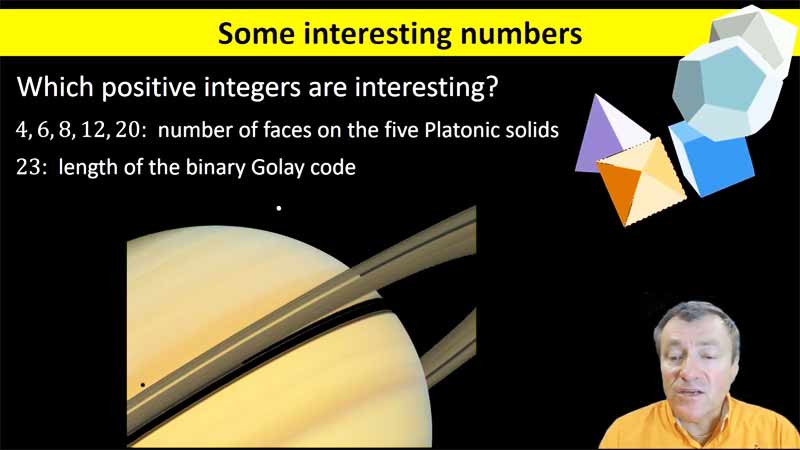 |
Which numbers are interesting? Are all numbers interesting? | |
| pp.21–22 | Q is Dense in R | 7:09 | 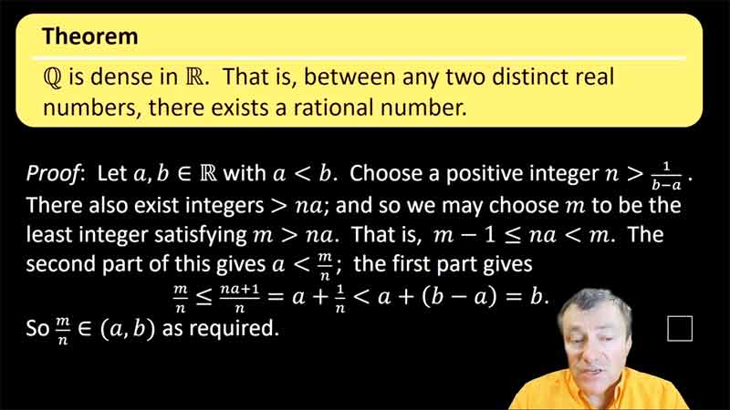 |
We prove the Archimedean property of the reals ('there are no infinite or infinitesimal real numbers'). We also prove that the rationals are dense in the reals. |
| pp.39–48 | Sequences | 15:45 | 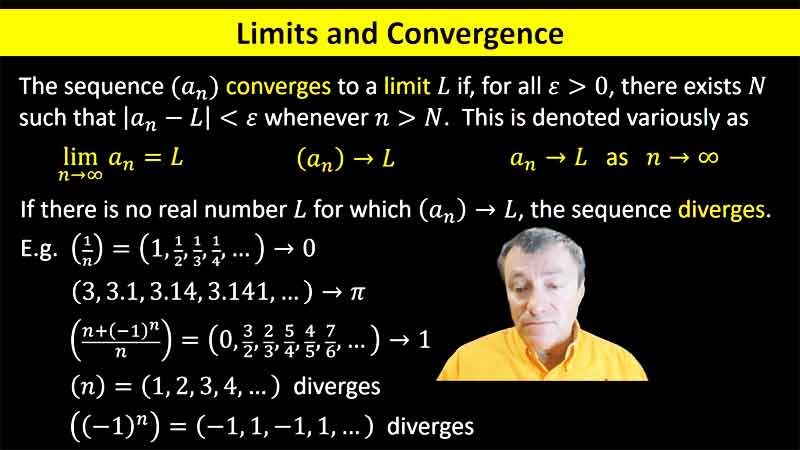 |
We discuss sequences of numbers and their properties (particularly limits, boundedness and monotonicity). The Monotone Convergence Theorem is presented, as another manifestation of the completeness of the real numbers. |
| pp.49–52 | Algebra with Sequences | 8:17 | 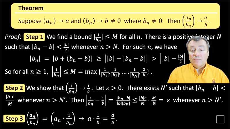 |
For algebraic operations on convergent sequences (term-by-term addition, multiplication and division) we prove that the resulting sequences are also convergent with limits as predicted by the familiar limit laws. |
| pp.1–4, Ex. 2.4.5 | A Discrete Dynamical System | 8:45 | 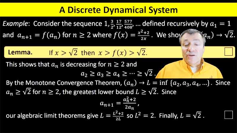 |
We consider a special instance of a recursively defined sequence whose terms are given by iterating a fixed map f. Here we obtain a sequence of rational numbers converging quadratically to sqrt(2). |
| pp.56–58 | Order with Sequences | 12:34 | 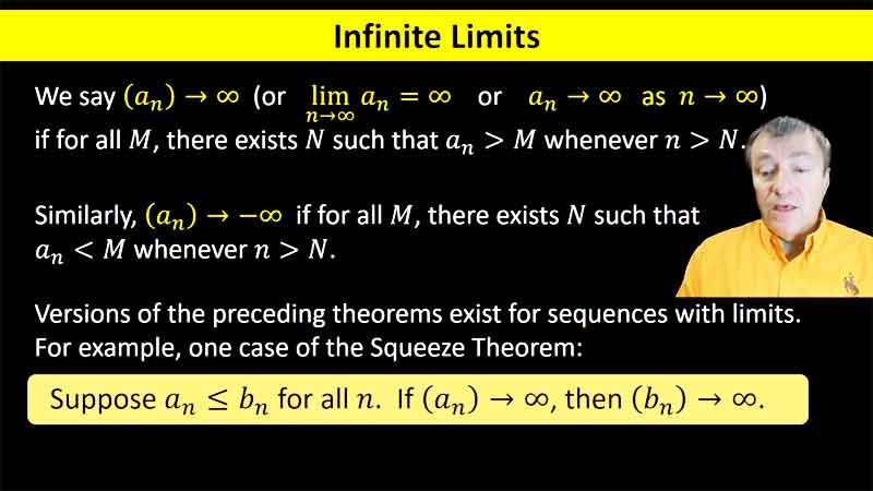 |
For convergent sequences whose terms satisfy certain inequalities, the limits also satisfy the expected inequalities. |
| pp.71–79 | Series | 23:44 | 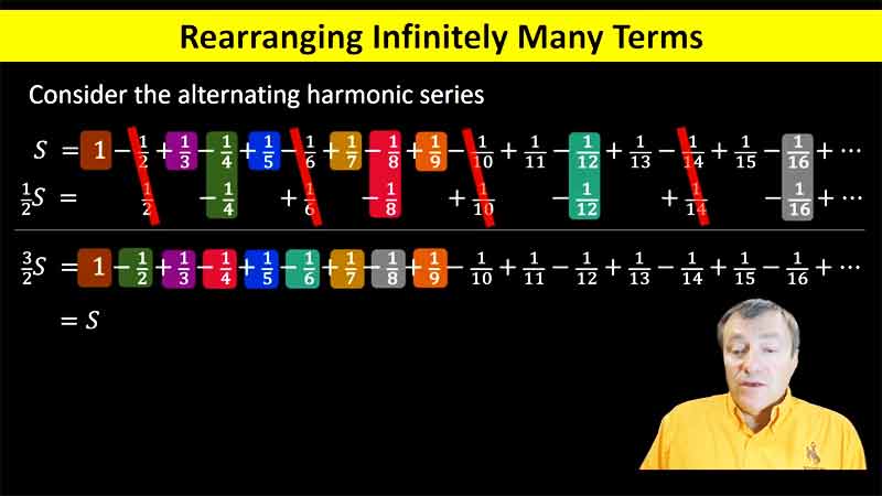 |
We define convergence of a numerical series, and discuss the extend to which its convergence may be altered by various modifications to the series, particularly rearrangements. |
| Stacking Bricks | 14:39 | 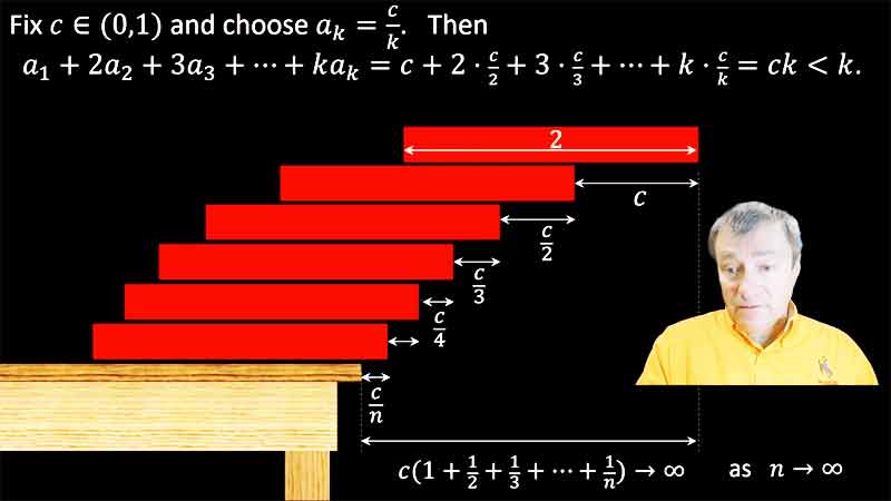 |
As a concrete interpretation of the divergence of the harmonic series, we discuss how far a stack of bricks can be made to extend beyond the edge of a table. | |
| pp.62–66 | Subsequences | 13:09 | 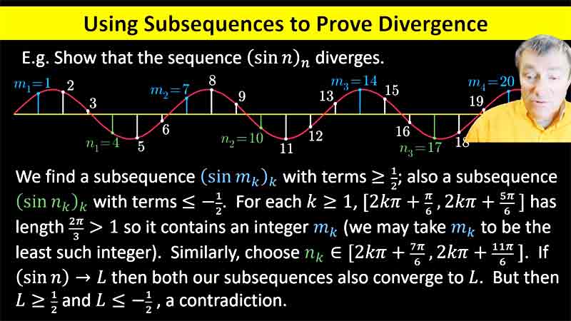 |
We discuss subsequences of sequences and their properties and uses. We show how subsequences can be used to prove divergence of a sequence. We also prove the Bolzano-Weierstrass Theorem: Every bounded sequence of real numbers has a convergent subsequence. |
| pp.66–68 | Cauchy's Criterion | 23:46 | 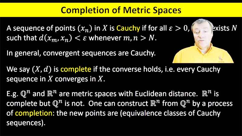 |
We discuss the notions of Cauchy sequence, metric spaces, and completeness. A metric space is a space with a reasonable notion of distance between points. The space is complete if every Cauchy sequence in the space converges. We show that that the real number system is complete. |
| pp.68–69, 297–298 | Foundations for R | 18:22 | 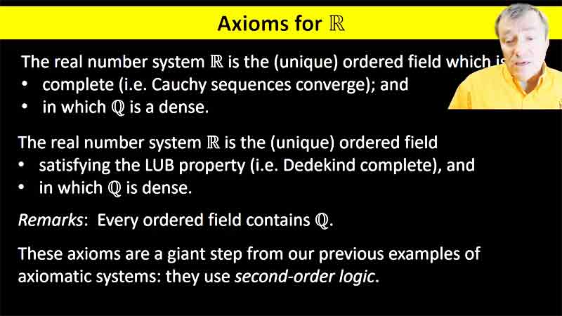 |
We finally give a set of axioms for the real number system: it is the unique complete ordered field in which the rationals are dense. We also compare the two most popular constructions of the reals from the rationals: either by completion in the metric space sense, or via Dedekind cuts. |
| pp.46, 63 | Divergent Series | 19:04 |  |
The controversy around Ramanujan's Summation provides us an opportunity to talk about divergent series, and whether or not they can be assigned values. This video (and its sequel) are not appropriate for students in calculus. |
| Normed Fields | 22:20 | 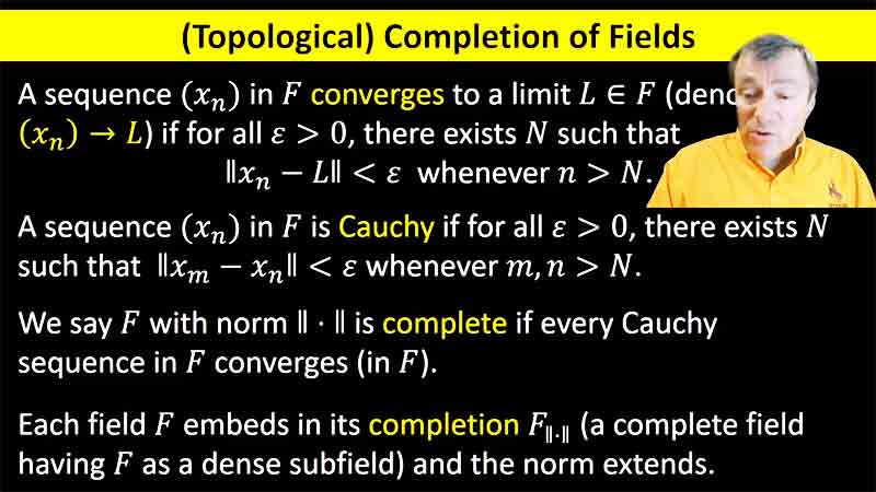 |
A hugely important theme in analysis is that of normed spaces (a special kind of metric spaces). One particular instance of this is normed fields, which we define here. Properties of sequences (including boundedness, convergence, and completeness) are generalized to this setting. | |
| pp.88–95 | Open and Closed | 17:00 | 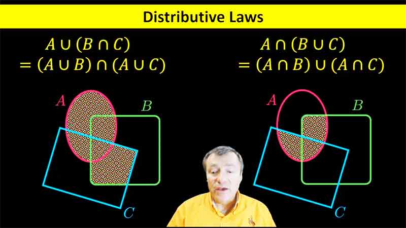 |
This is a brief introduction to the standard topology of the real number line, in which we define open and closed sets in the reals, and we give some of their most basic properties. We finish by showing that the real line is topologically connected. |
| pp.88–95, 104–106, 258 | Topology | 29:21 | 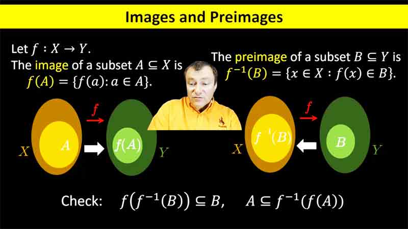 |
We define topological spaces, showing that these notions give a very short proof of the Intermediate Value Theorem. |
| pp.88–95 | Closure | 16:46 | 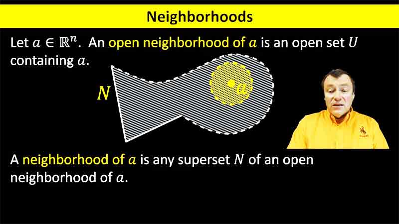 |
Several related topological notions are introduced: neighborhoods of points, limit points, and closure of point sets. |
| pp.97–99 | Compactness | 21:12 | 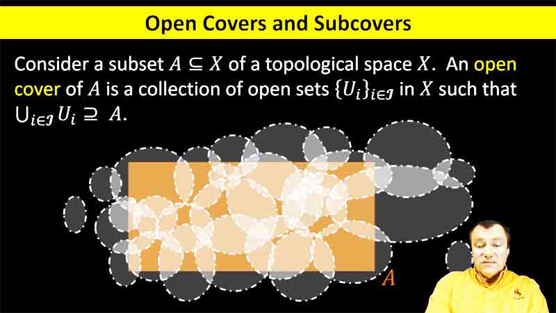 |
We define the topological property of compactness, and prove the Heine-Borel Thoerem: A subsets of the reals is compact iff it is closed and bounded. |
| pp.96–97 | Sequential Compactness | 4:31 | 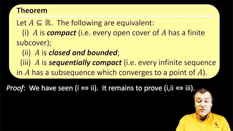 |
We show that for subsets of the real line, the property of sequential compactness (every sequence has a convergent subsequence) is equivalent to compactness. |
| pp.115–119 | Limits of Functions | |||
| O-notation | ||||
| pp.130–133 | Uniform Continuity | |||
| pp.173–178 | Uniform Convergence | |||
|
|
|
other Handouts
|
|
|
 / revised January, 2021