

Instructional videos for Math 2200 will be hosted on YouTube as linked in the table below.
Want more of these? Check out my colleagues' Math 2200 videos. Marissa Hegy posts her lectures on the YouTube channel MarissaHegyMath. And Bryce Christopherson posts at https://www.youtube.com/channel/UC3xFa71YnkIbaW1w5_mBrwQ
|
Textbook
|
Title
|
Duration
|
Link
|
Description |
|
§ 3.11
|
6:39 | Introduction to calculus problems regarding related rates (word problems using the chain rule). We discuss the setup; subsequent videos give examples. | ||
|
§ 3.11
|
11:50 | A first example of related rates: Air is pumped into an inflatable balloon at a rate of 10 in^3/sec. How fast is the diameter increasing at the moment when the diameter is (a) 5 in; (b) 10 in? | ||
|
§ 3.11
|
8:24 | Continuing our example of a first related rates problem in calculus | ||
|
§ 3.11
|
15:03 | We discuss three slightly different solutions to the following related rates problem: An airplane flies due west at an altitude of 1mi. Shortly after passing directly over our heads, it passes over the nearest town 1.4 miles to our west. Assuming the plane has groundspeed 540mph at that instant, how fast is the plane receding from us? | ||
|
§ 3.11
|
10:33 | Sequel to our previous video, Airplane I. Here we solve another related rates problem in calculus: An airplane is 1.4mi due west of us, flying due west at an altitude of 1mi. We observe its angle of inclination above the horizon. Assuming its groundspeed at that instant is 540mph, what is the rate of change of the angle of inclination? | ||
|
§ 3.11
|
||||
|
§ 4.1
|
Maxima and Minima | 23:08 | 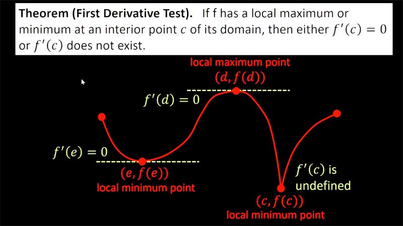 |
We introduce the notion of extrema (maxima and minima) for functions in single-variable calculus. |
| § 4.2 | Mean Value Theorem I | 8:30 | 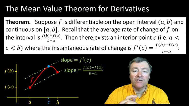 |
The Mean Value Theorem for Derivatives (together with Rolle's Theorem) are introduced. |
| § 4.2-4.3 | Mean Value Theorem II | 13:34 |  |
The Mean Value Theorem is used to test when a function is constant (or increasing or decreasing). We also discuss when two functions can have the same derivative. |
| § 4.3 | The Derivative Tests | 27:44 | 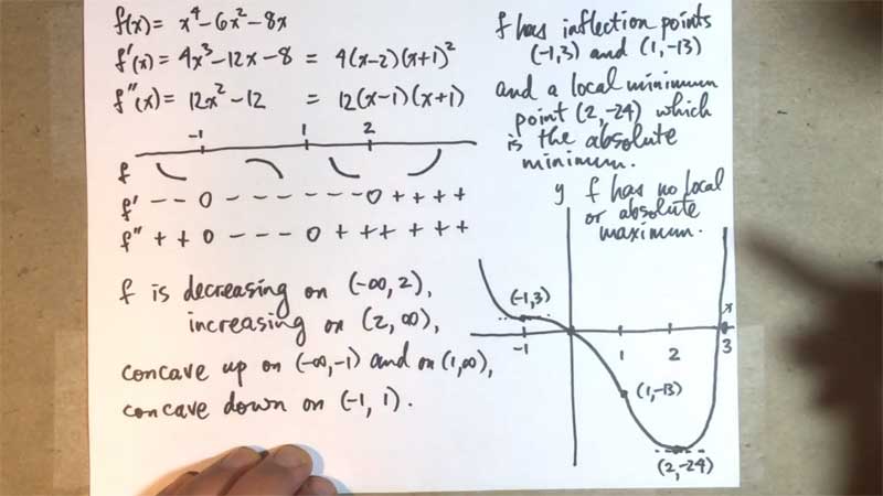 |
The First and Second Derivative Tests are introduced, whereby we determine intervals where a graph is increasing or decreasing, concave up or concave down. Example 1 (at 8:11) considers |
| § 4.3 | Some Fabulous Polynomials | 12:48 |  |
A remarkable sequence of polynomials is exhibited. Using the First Derivative Test, it is easily shown that these polynomials give lower bounds for ex (for x > 0). An application is given to evaluating certain limits. |
| § 4.4 | Sketching Graphs I | 13:10 |  |
We apply tools from calculus together with tools from pre-calculus in the art of sketching graphs of functions. At 6:27 we demonstrate using f(x)=(x2+36)/2x. |
| § 4.4 | Sketching Graphs II | 7:17 | 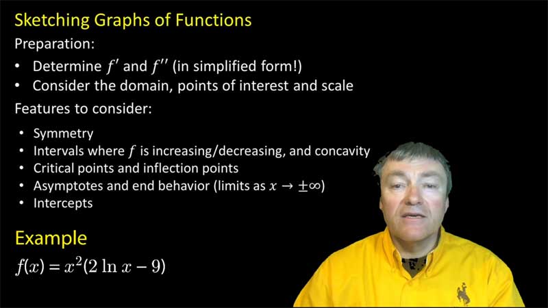 |
As a second example, we sketch the graph of f(x)=x2(2ln(x)-9). |
| § 4.5 | The Largest Box | 5:11 | 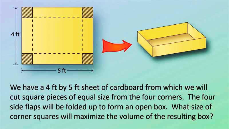 |
From a 4ft by 5ft sheet of cardboard, we cut squares of equal size from the four corners. This leaves four flaps on the sides which fold up to yield a box with an open top. What size of square cutouts from the corners will maximize the volume of the resulting box? |
| § 4.5 | The Shortest Ladder | 7:11 |  |
We want to lean a ladder against the outside wall of our house. What is the shortest possible ladder we can use if the ladder must reach over the top of a 6 ft tall fence which is 4 ft from the wall? |
| § 4.6 | Linearization and Differentials | 22:05 | 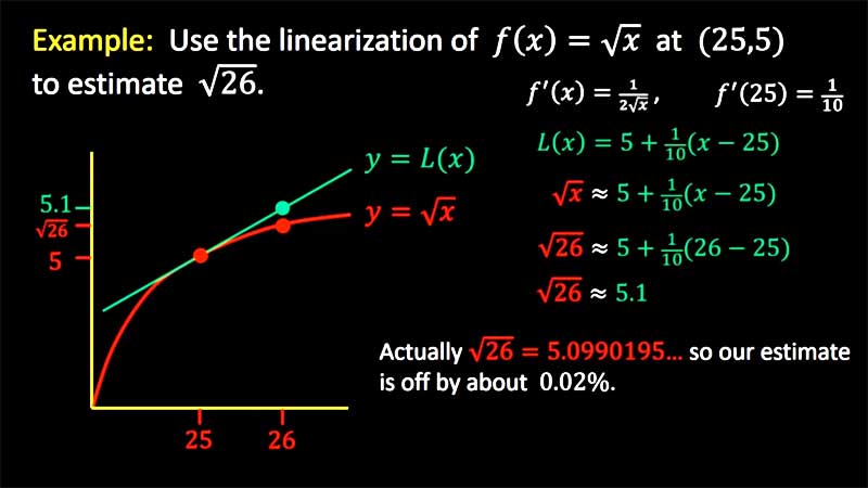 |
We discuss the linear approximation to a function at a point of its graph. At 12:05 we introduce differentials and discuss several ways they are used. |
| § 4.7 | l'Hôpital's Rule | 25.59 |  |
We explain how l'Hôpital's Rule is used to evaluate limits of indeterminate forms. Many examples (having different indeterminate forms) are included. |
| § 4.7 | Why the interest in e? | 12:31 |  |
The exponential function ex and the natural base e are shown to arise naturally in the context of continuously compounded interest. This uses l'Hôpital's Rule to resolve yet another indeterminate form. |
| § 4.9 | Antiderivatives I | 23:27 |  |
Antiderivatives are introduced. If f is the derivative of F (i.e. F′ = f ) then F is an antiderivative of f. |
| § 4.9 | Antiderivatives II | 15:02 | 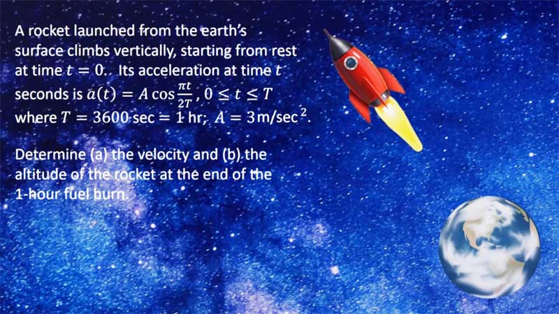 |
We continue discussing antiderivatives. At 5:25 we solve a problem: A rocket launched from the Earth's surface climbs vertically, starting from rest at time t=0. Its acceleration at time t seconds is a(t)=A cos(πt/2T) where T=1 hr and A=3m/sec2. Determine (a) the velocity and (b) the altitude of the rocket at the end of the 1-hour fuel burn. |
| § 5.1 | Riemann Sums I | 26:34 | 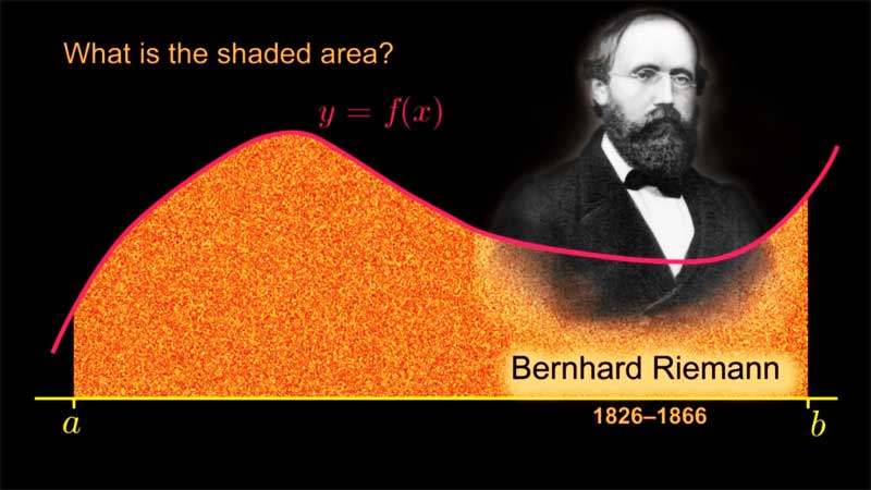 |
We introduce Riemann sums as approximations to areas under curves; and by taking the appropriate limit, we arrive at the definition of a Riemann integral. |
| § 5.1 | Riemann Sums II | 6:23 | 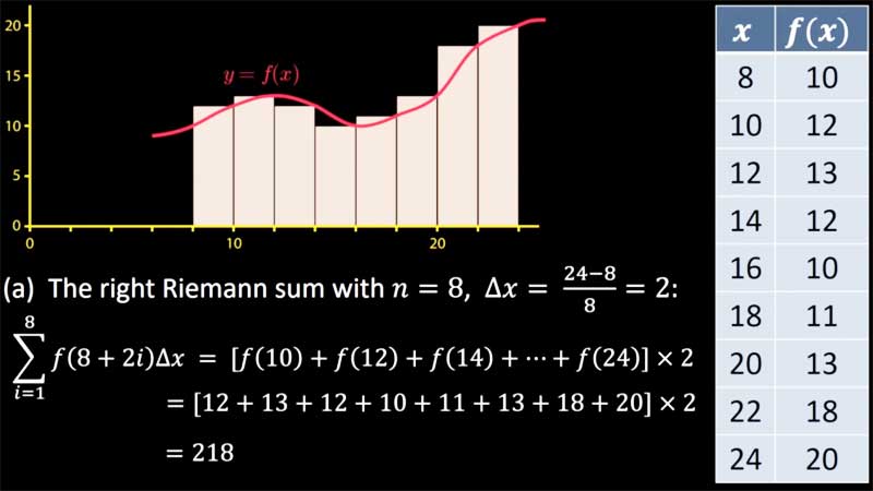 |
Using a table of values for a function, we compute left, right and midpoint Riemann sums using n=8,8,4 subintervals respectively. |
| § 5.1 | Riemann Sums III | 8:52 | 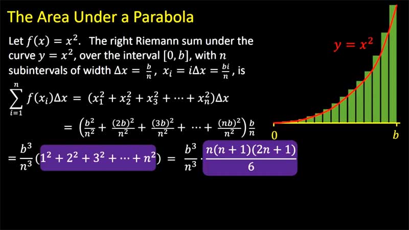 |
We evaluate two integrals using the definition (as the limit of Riemann sums) just for the functions f(x)=x and x2. |
| § 5.2 | Integrals | 13:52 | 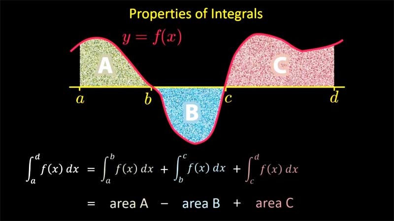 |
We cover the most basic properties of integrals, and their relationship with area. |
| § 5.3 | Fundamental Theorem I | 13:28 | 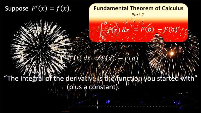 |
The Fundamental Theorem of Calculus is introduced in both its forms. |
| § 5.3 | Fundamental Theorem II | 11:36 | 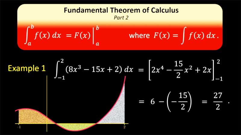 |
Examples using Part 2 of the Fundamental Theorem of Calculus. |
| § 5.3 | Fundamental Theorem III | 13:01 | 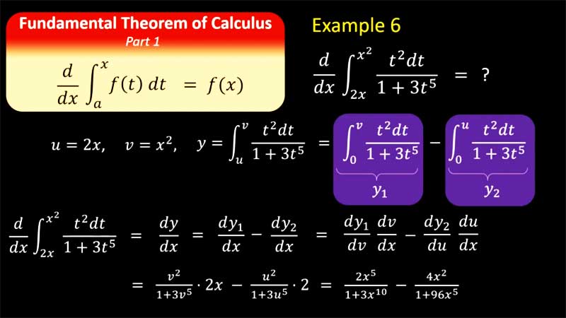 |
Examples using Part 1 of the Fundamental Theorem of Calculus. |
| § 5.4 | Average Value of a Function | 18:51 |  |
We define the average value of a function on an interval. We also discuss the use of symmetry in computing integrals. |
| § | ||||
| § |
 / revised April, 2020